Torque & Drag Simulations
It is difficult to give a recommendation on a general basis of which options to use for a specific analysis. Below is a detailed description of the effect of each option, which should help you on the way to select the correct option for your operation/simulation. Please read the NB's as they try to give some practical advice if you get unexpected results.
1. Piston Effect
When no piston effect is applied the buoyancy is calculated and applied to the weight of each drill string component. The buoyancy is the sum of all the forces caused by the pressure in the liquid acting on the component. Since the drill string components have dimensions > 0 the summed force/buoyancy is a force that is applied to the center of mass for the component. The buoyancy calculation does not show the compressive nature of pressure acting on the component in the tension plot. This is referred to as “Effective tension”.
By applying/selecting the piston effect option, the simulation is done by calculating the force from the pressure in the liquid acting on all the surfaces of the drill string. For tension analysis this means finding all the surfaces that are perpendicular to the axial vector of the drill string. Each force is applied at the geometric point at which it acts. The tension plot will thus also show the internal axial compression each component is subjected to. By applying piston forces the tension result is called “True tension”.
NB: If the effective and true tension plots have a high degree of deviation one of the common culprits is that the material density does not match the volume and weight of one or more components. The density only depends on the material used and should be standard. The weight is easy to measure, but the geometry can in many cases be the culprit of such a deviation. A simple, approximate method to get a matching result of density vs material volume vs component geometry, is to manipulate the length of the connector of the component in question.
2. Pipe in Pipe Friction model
Pipe in pipe friction model - The friction factor was reported in “Field method of assessing borehole friction for directional well casing” - Maidla and Wojtanowicz, Is dependent on radius of the casing and the drill string. Selecting this box the friction factor will be modified according to the geometry at the position at which the friction is calculated. This is a minor change to the friction factor supplied by the user, but the change is not constant in a moving mode analysis, as a drill pipe section will move through different diameter casings.
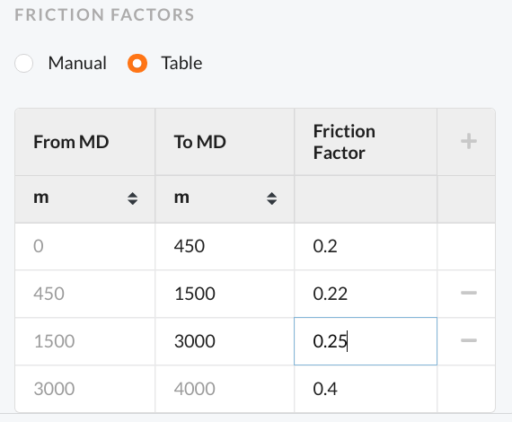
This option is a fine tuning of the results. This means that all geometric and mass input parameters needs to be accurate, for this effect to actually move the result closer to real life forces on the drill string. If the drill string runs through a casing with a constant diameter from "top" to "bottom", the effect is the same as changing the friction factor for "Casing", ie all friction on the casing is modified by a constant factor. On the other hand, if there are liners with decreasing diameters as the drill string moves down the well, the modification will be proportional to the diameter of the casing at "point of calculation". The same effect can be achieved by selection "Friction - Table" option, where the friction factor can be set to be valid only between specified MDs:
3. Soft 3D Model
Soft 3D model is a 3-dimensional modification to the Johancsik soft string model. Deemed to be a slightly more accurate calculation at the locations where the dogleg changes. The modification is used in all sections where the dogleg is non-zero. It depends both on the azimuthal and inclination changes. The model interprets the trajectory on a similar way as a "Stiff string" model. Thus this forms part of a hybrid model simulation. Selecting this option will have a higher impact on trajectories with tortuousity enabled than those without.
4. Pipe Bending Force Absorption
Pipe bending force absorption - Hybrid model, taking into account that the drill string is stiff/elastic. The drill pipe will bend through all parts of the well with a non-zero dogleg. To bend the pipe, a bending force needs to be applied to both ends of the pipe (compressive or tensional). When the pipe has the same dogleg as the curvature of the trajectory it will not bend any more as it will be supported by the wall. As long as the bending does not go beyond the yield strength of the metal, an opposing force from the pipe will equal the force needed to bend the pipe. When selecting this option, this force is taken into account in the calculation of all the forces acting on the drill string. Since the bending of the metal acts as a spring, some energy is thus stored, and the force that propagates to the next section is changed accordingly.
The overbending sub-option takes into account that the pipe can be bent even more than the dogleg of the trajectory if it has connectors with a diameter that is bigger than the pipe.
The effect of this calculation increases with the severity of the doglegs The highest modification will be seen on trajectories that has severe random tortuosity enabled.
5. Buckling Factors
A theoretical buckling force is calculated. This is an unstable equilibrium limit, thus in reality buckling happens typically when the compressive exceeds this but a “factor”. The default factors are the recommended factors (see eg: “Buckling - The state of the art” - R.F.Mitchell). When the compressive force exceeds the theoretical value multiplied by the lateral factor, then the drill string goes into lateral buckling, and correspondingly for the other factors. If the drill string goes into helical buckling a different set of equations is used to calculate the frictional force (see R.F.Mitchell paper).
6. Simulation Temperature
This menu specifies which temperature profile (temperature as s function of MD) to use in the simulation. The simulation can use a temperature profile inside the drill string that is different than the profile in the annulus (see "WellTemp simulation"). One of the following options can be selected:
- Geothermal: The density of drilling mud depends on the pressure and temperature. By selecting the geothermal temperature in this menu, the geothermal temperature will be used as the temperature of the mud inside the drill pipe and in the annulus, ie the same temperature. This would simulate a situation where the mud has been standing still, long enough for the mud to come into thermal equilibrium with its surroundings.
- BHCT: “Bottom Hole Circulating Temperature” is a model described in API RP 10B-2. This model is only valid when the drill string is longer than 3050 meters. Oliasoft has made a linear extrapolation when the drill string is shorter. At a point this breaks down, yielding temperatures that are lower than the geothermal temperature. In such a case the temperature is assumed to be the geothermal temperature. The model was based upon data from a series of near vertical wells, to be used for casing loads simulations. Highly deviated wells/long horizontal sections in a well, will not get a realistic temperature profile using this.
- WellTemp Simulation: See the well temp simulation page for more details. When selected, a full temperature simulation is done and used as input to the T&D simulation. This will give one temperature profile inside the drill string and another temperature profile in the annulus. They are much more realistic than the 2 other options in a situation where the mud has been circulating for a while.
NB: Using the correct temperature profile for your simulation is extremely important wrt the density (and ECD in hydraulics) calculations. Most drilling muds have a thermal expansion coefficient that combined with a high temperature gradient will easily exceed the compressibility coefficient compared to pressure gradient in the well. If the density looks "inverted" make sure you are using the desired simulation temperature profile.